Statistics for Online Platforms
A Statistical Analysis for
Interleaving Design in A/B Tests
Weitao Cheng, Ningyuan Chen, Pin Gao, Nian Si
HKUST IEDA
INFORMS November 2026
Background
A/B tests
Is B $>$ A, statistically significantly?

Thousands of A/B tests are conducted on online platforms each day.
Background
Online (two-sided) platforms: e-commerce








✓
✓

✓
✓

✓
Background
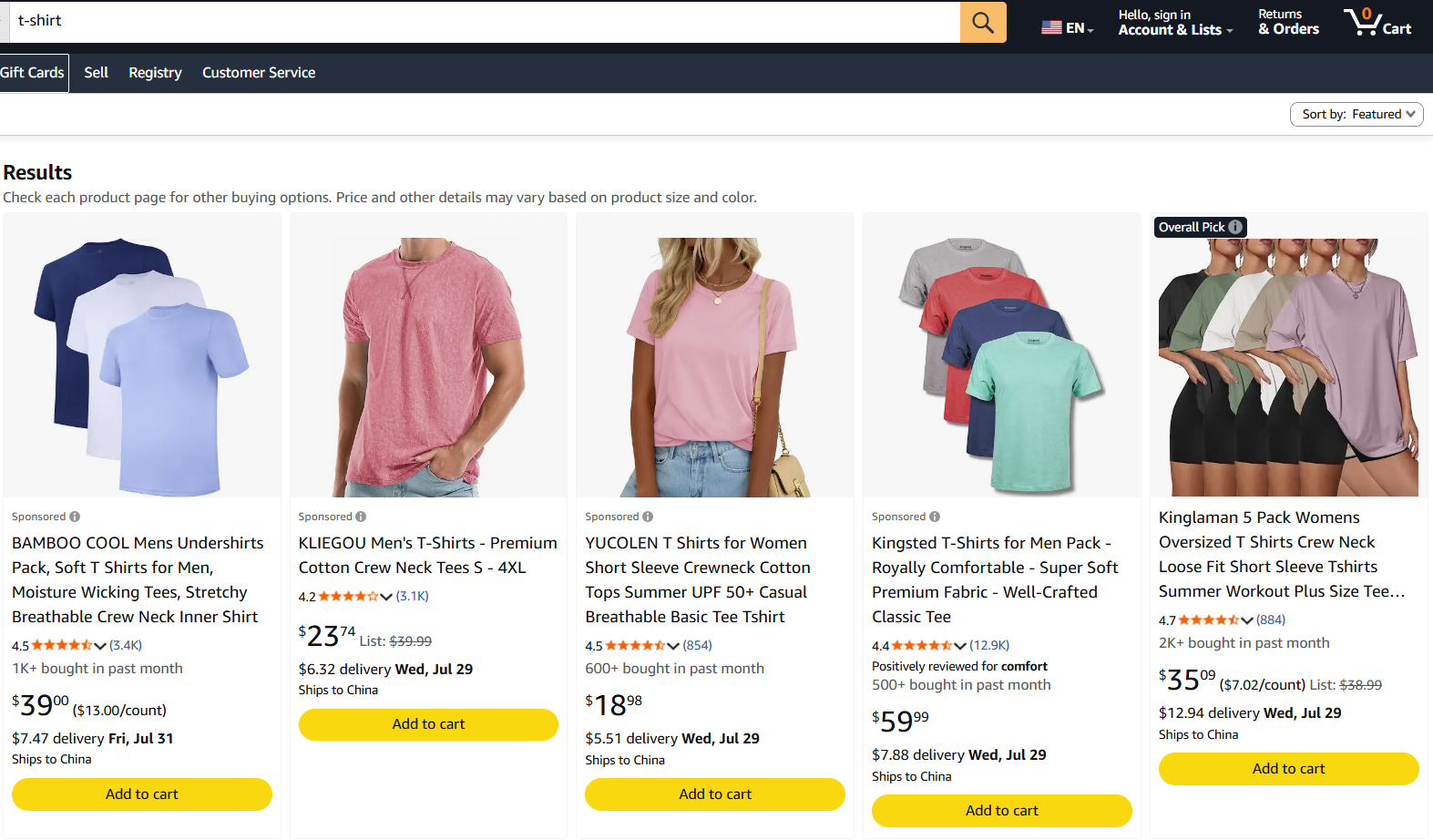
A/B testing Assortment (slate) recommendation I: e-commerce
Control
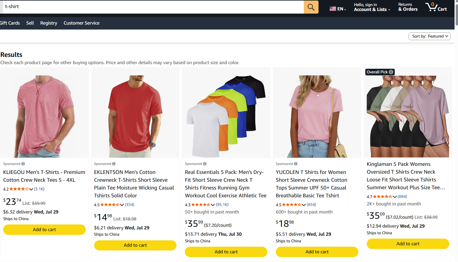
Treatment
Background
A/B testing Assortment (slate) recommendation II: content feed
Control

Treatment

Research Question
Research Question
Can we design experiments and estimators that optimally (A/B) test assortment recommendation policies?
- Maximize power while controlling type-I error
- Optimal experimental design and optimal estimators
$$\begin{aligned} \max_{\text{design},\ \text{estimator}} \quad & \text{power} \\ \text{s.t.} \quad & \text{type-I error} \le \alpha \end{aligned}$$
Agenda
- I. Interleaving Estimators
- II. Base Model: Homogeneous Users and Assortments
- III. Heterogeneous Users and Assortments
- IV. Numerical Experiments
I — Interleaving Estimators
Two ways to compare assortment policies
- User-side experiment (UE): randomize each user to see one full assortment, $S^T$ or $S^C$.
- Unbiased but can be high variance.
- Interleaving design (IE): merge $S^T$ and $S^C$ into a single assortment $S^I$ shown to every user.
- High sensitivity but not automatically valid.
- How to optimally interleave?
User-side experiment
$S^T$
→
$S^C$
→
Interleaving design (one possibility)
$S^T$
$S^C$
→
→
I — Interleaving Estimators
Some possible interleaving designs
$S^T$
$S^C$
→
Full union: everything from both sides
$S^T$
$S^C$
→
Symmetric difference: exclusive items only
$S^T$
$S^C$
→
Balanced design: one random item from each side, plus the shared items
$S^T$
$S^C$
→
50%
50%
No-share mixing experiments: exclusive terms each w.p. $1/2$: no sharing
II — Base Model
Users, items, and the choice model
- $N$ users $[N]$, $M$ items $[M]$, outside option $0$; $S_+ = S\cup\{0\}$ for any assortment $S\subseteq[M]$.
- $Y_{ij}(S)\in\{0,1\}$: potential outcome — whether user $i$ selects item $j$ under assortment $S$.
- Treatment/control assortment policies $S^T$, $S^C$.
- Item partition: $A^T=S^T\setminus S^C$, $A^C=S^C\setminus S^T$, $A^S=S^T\cap S^C$, with $|A^T|=|A^C|=:r$ and $|S^T|=|S^C|=:m$.
$S^T$$S^C$$A^T$$A^S$$A^C$
- Choice model:
Multinomial logit (MNL)$$P(j \mid S) = \dfrac{w_j}{1+\sum_{k\in S}w_k},\ \ j\in S_{+},\quad w_j>0,\ w_0=1$$
Items compete through a shared denominator. A user selects at most one item.
II — Base Model
The demand effect and the testing problem
- Estimand. The average treatment effect on demand — the difference in expected demand per user between the two policies: $$\mathrm{ATE}^{D} := D(S^{T}) - D(S^{C}),$$ where $D(S) := \mathbb E\bigl[\sum_{j\in S} Y_{ij}(S)\bigr] = \sum_{j\in S} P(j\mid S)$ is the expected demand per user when $S$ is offered.
- Testing problem. Decide whether the treatment policy changes demand at all: $$H_{0}^{D}: \mathrm{ATE}^{D} = 0 \quad \text{versus} \quad H_{1}^{D}: \mathrm{ATE}^{D} \neq 0.$$
We focus on the sign of $\mathrm{ATE}^{D}$ — comparing algorithms, not estimating a level.
II — Base Model
The interleaving design space
- Assortment space $\mathcal B_{\mathrm{general}}=\{S^I: S^I\subseteq S^T\cup S^C,\ |S^I|\ge1\}$;
- An interleaving design $\xi \in \mathcal{P}(\mathcal B_{\mathrm{general}})$ is a probability distribution over it, with $S_i^I\overset{\mathrm{iid}}{\sim}\xi$.
- Symmetric-difference design: $S^I=S^T\triangle S^C=A^T\cup A^C$ (deterministic, $\xi_{S^I}=1$).
- Balanced design $\xi_B(k)$: uniform over $\{T\cup C\cup F: T\subseteq A^T,|T|=k,\ C\subseteq A^C,|C|=k,\ F\subseteq A^S,|F|=m-2k\}$.
- User-side experiment (UE) as a degenerate interleaving design: $\mathcal B_{\mathrm{user}}=\{S^T,S^C\}$, $\mathbb P(S_i^I=S^T)=\pi$.
The design space unifies UE and IE in a single framework.
II — Base Model
Estimators for both designs
- UE. Randomize $Z_i$; show $S^T$ if $Z_i=1$, else $S^C$. Denote $S_i^I(Z_i):=S^T$ if $Z_i=1$ and $S^C$ if $Z_i=0$. With $U_i=\sum_{j\in S_i^I(Z_i)}Y_{ij}$, the difference-in-means estimator is:
$$\hat\Delta_{UE}=\bar U_T-\bar U_C$$UE: difference-in-means
- IE. Show every user a merged assortment $S_i^I\subseteq S^T\cup S^C$, drawn i.i.d. from a design $\xi$; construct scores from the observed selections under the merged display.
$$Q_i:=\sum_{j\in A^T}Y_{ij}-\sum_{j\in A^C}Y_{ij}, \qquad \hat\Delta_{I,\mathrm{mean}}=\frac1N\sum_{i=1}^N Q_i$$
IE: simple mean
II — Base Model
CLT & power for both designs
User-side experiment (UE)
$$\frac{\hat\Delta_{UE}- \mathrm{ATE}^{D}}{\sqrt{\hat{v}_T/N_{1}+\hat{v}_C/N_{0}}} \xrightarrow{d} N(0,1)$$
CLT
Interleaving score
$$\frac{\hat\Delta_{I,\mathrm{mean}}-\mathrm E[Q_i]}{\sqrt{S^2/N}}\xrightarrow{d}N(0,1)$$
CLT
Both tests share the same asymptotic form — reject when $|Z|>z_{1-\alpha/2}$ — with approximate power $1-\Phi\!\bigl(z_{1-\alpha/2}-\sqrt N|\kappa|\bigr)$. $\kappa$ is the signal-to-noise ratio that governs power: our problem reduces to maximizing $\kappa_{I,\mathrm{mean}}(\xi)$.
$$\pi^{\star} = \frac{\sqrt{v_{T}}}{\sqrt{v_{T}} + \sqrt{v_{C}}}, \quad \kappa_{UE}(\pi^{\star}) = \frac{\mathrm{ATE}^{D}}{\sqrt{v_{T}} + \sqrt{v_{C}}}$$
optimal allocation
$$\kappa_{I,\mathrm{mean}}(\xi):=\frac{\mathrm E[Q_i]}{\sqrt{\operatorname{Var}(Q_i)}}$$
signal-to-noise ratio
II — Base Model
Valid design spaces & optimal design problem
- Valid design space. Design should output correctly under the null: $$\mathcal{D}(\hat{\Delta}) := \left\{\xi: \mathbb{E}_{\xi,w}[\hat{\Delta}] = 0 \iff \mathrm{ATE}^{D}(w)=0\ \text{ for all admissible } w\right\}$$
- Optimal design problem. Among valid designs, maximize the signal-to-noise ratio governing power: $$\max_{\xi\in\mathcal{D}(\hat{\Delta}_{I,\mathrm{mean}}) } \quad |\kappa_{I,\mathrm{mean}}|$$
II — Base Model
MNL: symmetric difference is valid and power-optimal
- Valid design space: a design is valid exactly when it treats the two sides as blocks and shows no favoritism —
- All or nothing: the treatment-only items appear as a whole block or not at all; same for the control-only items.
- No favoritism: whatever shared items are on display, showing "treatment block only" must be exactly as likely as showing "control block only".
- Optimal design — attained by symmetric difference $S_i^I=A^T\cup A^C$: $$\kappa^{\mathrm{MNL},\star}_{I,\mathrm{mean}}=\frac{|w_T-w_C|}{\sqrt{w_T+w_C+4w_Tw_C}},$$ where $w_T:=\sum_{j\in A^T}w_j$, $w_C:=\sum_{j\in A^C}w_j$ (shorthand used throughout).
Remark: $\left|\kappa_{I,\mathrm{mean}}^{\mathrm{MNL},\star}\right|\ge\left|\kappa_{UE}^{\mathrm{MNL}}(\pi^\star)\right|$ — optimal interleaving weakly dominates the best user-side design.
III — Heterogeneous Users and Assortments
homogeneous users
→
Heterogeneous Users
Heterogeneous Users and Assortments
Different users see different assortments and respond differently — does interleaving still win and what is the optimal estimator?
III — Heterogeneous Users and Assortments
Contextual choice models
- Contextual MNL (C-MNL). Each user carries a context $\mathbf X_i$, and attractiveness weights depend on it: $$P(j\mid S,\mathbf X_i)=\dfrac{w_j(\mathbf X_i)}{1+\sum_{k\in S}w_k(\mathbf X_i)},\ \ j\in S_+.$$
- Estimand. The context-conditional effect and its average over contexts: $$\tau^D(\mathbf X):=D(S^T(\mathbf X);\mathbf X)-D(S^C(\mathbf X);\mathbf X), \qquad \mathrm{ATE}^{D}=\mathbb E_{\mathbf X}[\tau^D(\mathbf X)],$$ where $D(S;\mathbf X_i):=\mathbb E\bigl[\sum_{j\in S}Y_{ij}(S)\mid\mathbf X_i\bigr]=\sum_{j\in S}P(j\mid S,\mathbf X_i)$ is the expected demand per user with context $\mathbf X_i$ when $S$ is offered.
- Generality. The contextual MNL choice model can approximate a wide range of choice models, including random utility models (McFadden and Train, 2000).
III — Heterogeneous Users and Assortments
Testing problem: sharp null and monotone treatment
- Sharp null. Under C-MNL, the weak null is sharpened: with $w_T(\mathbf X)=\sum_{j\in A^T}w_j(\mathbf X)$ and $w_C(\mathbf X)=\sum_{j\in A^C}w_j(\mathbf X)$, $$H_0^{s}:\ w_T(\mathbf X)=w_C(\mathbf X)\ \text{a.s.} \qquad H_1^{s}:\ \mathbb P_{\mathbf X}\{w_T(\mathbf X)\ne w_C(\mathbf X)\}>0.$$
- Monotone treatment.
Assumption 1 (Monotone treatment — one-sided dominance)
The treatment is monotone relative to the control if one of the following one-sided dominance conditions holds:
$$\mathbb P_{\mathbf X}\{w_T(\mathbf X)\ge w_C(\mathbf X)\}=1 \quad\text{or}\quad \mathbb P_{\mathbf X}\{w_T(\mathbf X)\le w_C(\mathbf X)\}=1.$$
Remark: Heterogeneous user preferences, but homogeneous treatment direction — users may differ arbitrarily in how much they like each item, as long as the treatment moves everyone in the same direction.
III — Heterogeneous Users and Assortments
Heterogeneity breaks the story: UE can beat interleaving
- Two contexts with probabilities $(0.1,\,0.9)$ and weights $(w_a,w_b,w_s)=(10,\,0.05,\,0.1)$ / $(50,\,49.95,\,1)$: symmetric-difference interleaving gives $\kappa_{I,\mathrm{mean}}\approx0.0917$, while the optimal UE gives $\kappa_{UE}^\star\approx0.167$ — strictly more powerful than interleaving.
Context $x_1$ — 10% of traffic
$w_T=10$
$w_C=0.05$
decisive — carries all the signal
Context $x_2$ — 90% of traffic
$w_T=50$
$w_C=49.95$
near-tied — pure noise, no signal
Sym-diff interleaving $\kappa_{I,\mathrm{mean}}$
0.0917
Optimal user-side $\kappa_{UE}^\star$
0.167
Intuition: the near-tied, high-traffic context contributes large interleaving noise but little signal; UE preserves the signal from the rarer, decisive context without paying that noise. Interleaving design is worse even under a monotone-treatment condition ($w_T(\mathbf X)\ge w_C(\mathbf X)$ a.s., or the reverse).
III — Heterogeneous Users and Assortments
Context reweighting: the optimization problem
- Estimator. Some contexts contribute a large share of the variance but little mean signal — so reweight the score by context. $$\hat\Delta_I^\gamma:=\frac1n\sum_{i=1}^n \gamma(\mathbf X_i)\,Q_i, \qquad \text{where } Q_i=\sum_{j\in A^T(\mathbf X_i)}Y_{ij}-\sum_{j\in A^C(\mathbf X_i)}Y_{ij} \text{ and } \gamma:\mathcal X\to[0,\infty).$$
- Optimization problem. Choose the nonnegative context weight maximizing the signal-to-noise ratio: $$\sup_{\gamma\in\Gamma_\xi}\ |\kappa_\gamma|, \qquad \text{where }\kappa_\gamma:=\frac{\mathbb E[Q_i^\gamma]}{\sqrt{\operatorname{Var}(Q_i^\gamma)}}, \qquad Q_i^\gamma:=\gamma(\mathbf X_i)\,Q_i,$$ over the admissible class $\Gamma_\xi:=\bigl\{\gamma:\mathcal X\to[0,\infty),\ 0<\operatorname{Var}(Q_i^\gamma)<\infty\bigr\}$.
III — Heterogeneous Users and Assortments
Jointly optimal design and estimator
- Maximize power over the design $\xi$ and the estimator $\gamma$ at the same time, where $\mu_\xi(x):=\mathbb E_\xi[Q_i\mid \mathbf X_i=x]$ and $m_{2,\xi}(x):=\mathbb E_\xi[Q_i^2\mid \mathbf X_i=x]$.
Theorem 1 (Jointly optimal interleaving design and context weight under C-MNL)
Suppose C-MNL and monotone treatment hold, $\xi$ is independent of $\mathbf X_i$, and $|A^T|=|A^C|\ge1$. Write $R_\xi:=\mathbb E_{\mathbf X}\bigl[\mu_\xi^2(\mathbf X)/m_{2,\xi}(\mathbf X)\bigr]$. Then, jointly over valid designs and nonnegative context weights,
$$\sup_{\xi\in \mathcal D_{\mathrm{MNL}}(\hat\Delta_{I,\mathrm{mean}})}\ \sup_{\gamma\in\Gamma_\xi}\ |\kappa_\gamma|^2=\frac{R_I^\star}{1-R_I^\star},\qquad R_I^\star=\mathbb E_{\mathbf X}\!\left[\frac{\{w_T(\mathbf X)-w_C(\mathbf X)\}^2}{\{w_T(\mathbf X)+w_C(\mathbf X)\}\{1+w_T(\mathbf X)+w_C(\mathbf X)\}}\right],$$
attained by the symmetric-difference design $S^I(x)=A^T(x)\cup A^C(x)$ together with the oracle context weight
$$\gamma^\star(x)\ \propto\ \frac{|\mu_\xi(x)|}{m_{2,\xi}(x)}\ \propto\ \frac{|w_T(x)-w_C(x)|}{w_T(x)+w_C(x)}.$$
Dominance restored: under monotone treatment, $\left|\kappa_{UE}^{\mathrm{C\text{-}MNL},\star}\right|\le\left|\kappa_{I,\mathrm{opt}}^{\mathrm{C\text{-}MNL},\star}\right|$ — the oracle-weighted optimal interleaving test has weakly larger power than the optimally allocated user-side experiment.
IV — Numerical Experiments
Numerical Experiments
Does the theory hold up in simulation — type-I error control and the power ranking?
IV — Numerical Experiments
Methods compared
| Method | Design and statistic |
|---|---|
| UE-DIM-Ora | User-side A/B randomization with the difference-in-means statistic and oracle-optimal treatment allocation. |
| UE-HT-Ora | User-side A/B randomization with the Horvitz–Thompson statistic and oracle-optimal allocation. |
| IE-SD | Deterministic symmetric-difference display, using the unweighted interleaving score $Q_i$. |
| IE-SD-Ora | Same display, weighted by $\gamma^\star(x)\propto |\mu_x|/m_{2,x}$ using population moments. |
| IE-SD-Est | For discrete contexts, estimate the conditional first and second moments of $Q_i$, then plug them into $\widehat\gamma(x)$. |
Common protocol: Tests are two-sided at $\alpha=0.05$, with $R=500$ replications and sample size $N\in\{500,1000,2000,5000,10000,20000\}$. Under the sharp null, IE-SD-Ora is omitted because its oracle weight is zero.
IV — Numerical Experiments
Contextual MNL: type-I error
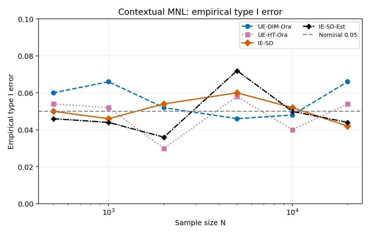
Type-I error: rejection rates stay around the nominal $0.05$ level.
IV — Numerical Experiments
Contextual MNL: power
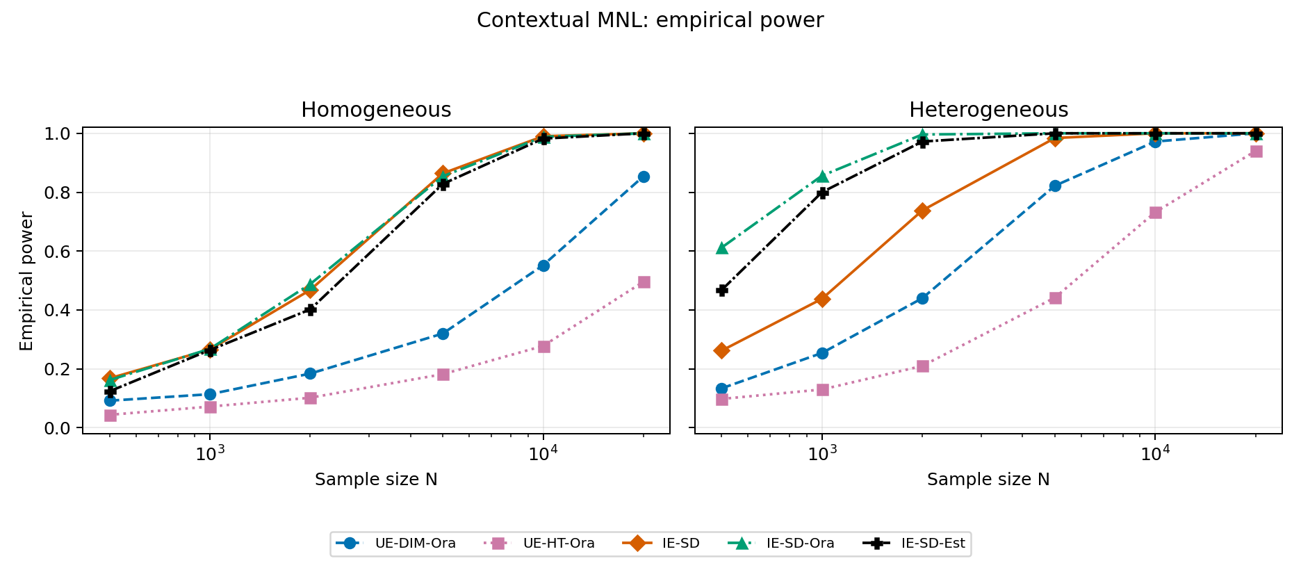
Power: interleaving substantially outperforms the user-side tests. As users become more heterogeneous , oracle weighting becomes especially valuable; IE-SD-Est recovers much of this gain as $N$ grows.
IV — Numerical Experiments
Contextual RUM: type-I error
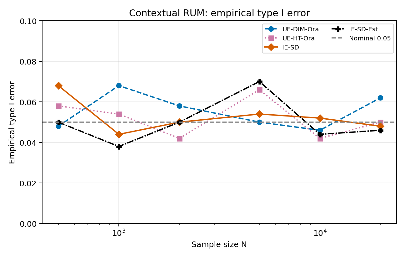
Type-I error: rejection rates stay around the nominal $0.05$ level.
IV — Numerical Experiments
Contextual RUM: power
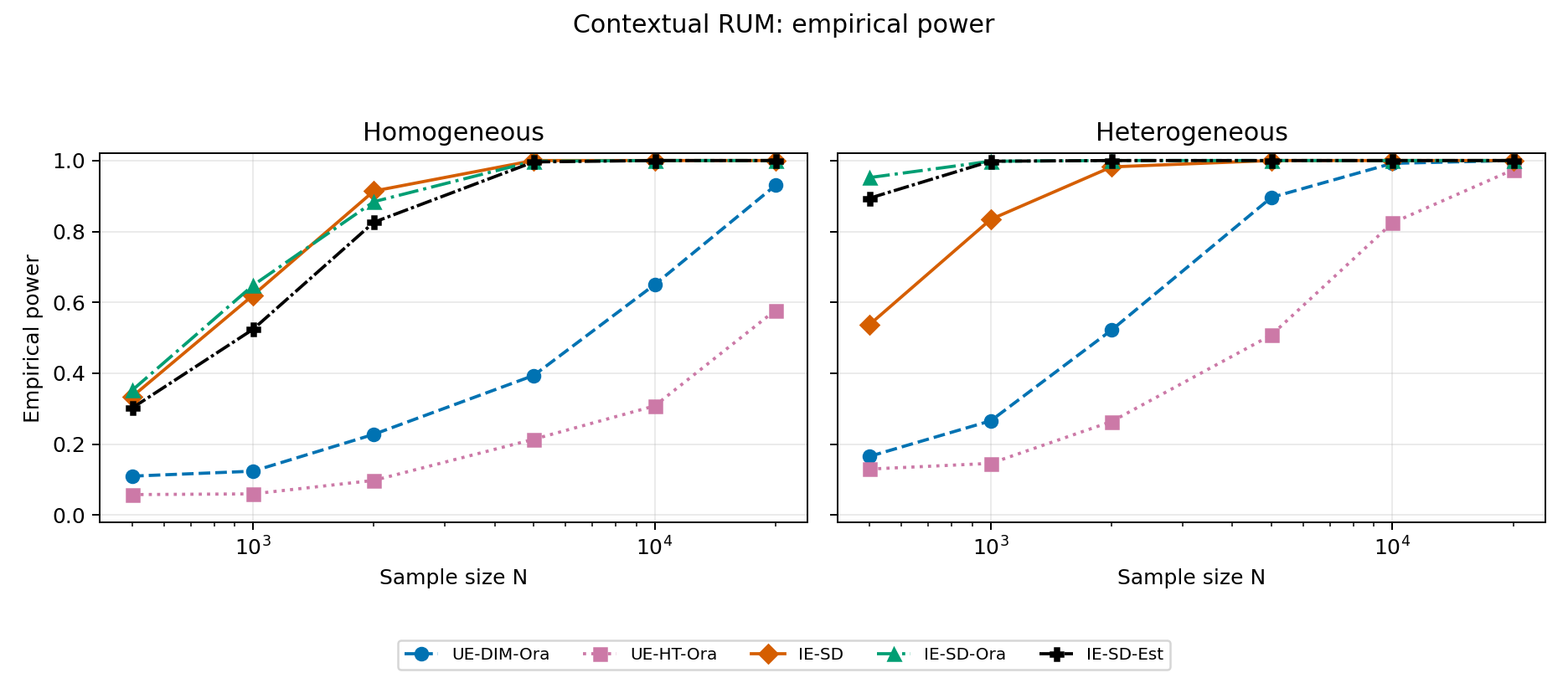
Power: the same qualitative advantage persists under contextual RUM with correlated Gaussian noise.
Summary
- Interleaving design is usually a valid and sample-efficient method for A/B testing, but not always.
- One should use weighted estimators if the users are too heterogeneous.
| Choice model | Design | Estimator | Optimal interleaving vs. UE |
|---|---|---|---|
| MNL | Symmetric difference | Simple mean $\hat\Delta_{I,\mathrm{mean}}$ | Interleaving $\ge$ UE |
| C-MNL | Symmetric difference | Simple mean $\hat\Delta_{I,\mathrm{mean}}$ | UE can beat interleaving |
| C-MNL | Symmetric difference | Context-reweighted $\hat\Delta_I^{\gamma^\star}$ | Interleaving $\ge$ UE |
Thank You — Questions & Discussion
Appendix
Appendix
Appendix
Why balanced designs fail under MNL
- Let $A^T=\{a,b\}$ with $(w_a,w_b)=(2,3)$, and $A^C=\{c,d\}$ with $(w_c,w_d)=(1,4)$. Since $\sum_{A^T}w_j=\sum_{A^C}w_j=5$, we have $\mathrm{ATE}^{D}=0$.
- Under the balanced design with $r=2,k=1$, direct computation gives $$\mathbb E_{\xi,w}[Q_i]=\frac{67}{1120}>0.$$
- The simple-mean interleaving score is biased away from zero exactly at the null — positive inclusion probabilities alone do not restore validity.
Once items compete through a shared MNL denominator, giving every exclusive item a positive chance of being displayed is not enough — the design must also satisfy the all-or-nothing and no-favoritism conditions.
Appendix
Simulation setting
A stylized search platform
- Let $X\in\{\mathrm{HF},\mathrm{MF},\mathrm{LT}\}$ denote high-frequency, medium-frequency, and long-tail queries, arriving with probabilities $(0.5,0.3,0.2)$.
- Each policy recommends one exclusive item: $S^T(x)=\{a_x\}$ and $S^C(x)=\{b_x\}$; interleaving displays both. This removes shared-item variation and isolates context heterogeneity.
- Baseline utilities $(\beta_{\mathrm{HF}},\beta_{\mathrm{MF}},\beta_{\mathrm{LT}})=(1,0,-1)$ make engagement highest for frequent queries and lowest for difficult long-tail queries.
What varies in the simulation?
- The treatment lift is $\Delta v(x)=\lambda d_x(\eta)$, where $d_x(\eta)=1+\eta h_x$ and $(h_{\mathrm{HF}},h_{\mathrm{MF}},h_{\mathrm{LT}})=(-1/2,0,5)$.
- $\lambda$ controls the overall effect size: $\lambda=0$ is the sharp null; power results use $\lambda=0.10$.
- $\eta$ controls where the gain occurs: $d_x(0)=(1,1,1)$, while $d_x(1)=(0.5,1,6)$ concentrates the improvement on rare long-tail queries.
Economic meaning: can context-aware interleaving exploit large improvements on rare, difficult queries without losing type-I-error control?
Appendix
How contextual utilities generate choices
Shared systematic utilities: $v_a(x)=\beta_x+\lambda d_x(\eta)$, $v_b(x)=\beta_x$, and $v_0(x)=0$. A user chooses the largest random utility $U_{j,x}=v_j(x)+\varepsilon_j$, where $j\in\{a,b,0\}$ and $0$ is the outside option.
Contextual MNL
- The shocks $\varepsilon_a,\varepsilon_b,\varepsilon_0$ are independent and identically distributed Type-I extreme-value (Gumbel).
- Thus $\Pr(j\mid x)=\exp\{v_j(x)\}/\sum_{k\in\{a,b,0\}}\exp\{v_k(x)\}$.
- Independent shocks make this the IIA benchmark.
Contextual Gaussian RUM
- $(\varepsilon_a,\varepsilon_b)$ are standard Gaussian with $\operatorname{Corr}(\varepsilon_a,\varepsilon_b)=\rho=0.5$; $\varepsilon_0$ is independent standard Gaussian.
- Choice probabilities are $\Pr\!\left(U_{j,x}=\max_k U_{k,x}\right)$, evaluated by Gauss–Hermite quadrature.
- Correlated item shocks allow the two recommendations to move together, relaxing IIA.